In this post I outline a way of simulating movement on a grid in R in a time efficient way. This is part of a simulation of tsetse fly populations I’ve been developing. Earlier posts outline some of the background and use of arrays as the main data structure.

My remit is to recreate in R an existing simulation developed in Excel (Hat-trick) which represents a fly population on a square grid of different vegetation types. In the Excel simulation tsetse flies are represented as moving to one of the 4 cardinal neighbouring cells. The boundaries of the square area are considered to be reflective, thus assuming that cells outside of the area are similar to their neighbours within the area. Movement is also represented as being dependent upon the age & sex of flies and the vegetation within cells.

A long time ago I wrote simulations of the movements of beavers and raptors but they were in C and based on looping through cells. Initial reading suggested that looping in this way in R would be very slow. I then came across this nice blog post by Petr Keil : Fast Conway’s game of life in R. In it he demonstrates a quick way of simulating movement that takes advantage of R’s efficient matrix operations.

A mechanism for simulating movement on a grid

1. create a shifted copy of the grid for each direction that you want to allow movement in (4 grids if NSEW, 8 grids if including diagonals).
2. calculate the number of arrivers in all cells on the grid by
   • adding the grids together
   • multiply by the proportion moving
   • divide by the number of neighbours (4 if NSEW, 8 if including diagonals)
3. calculate the number staying in all cells by multiplying the original grid by 1 minus the proportion moving
4. get the new distribution by adding the grids for arrivers and stayers

This is the bare code for an island model in which no movers come in from outside and any leaving are lost to the population:

#create a starting matrix and proportion moving
  m <- matrix(c(0,0,0,0,1,0,0,0,0),nrow=3,ncol=3)
  pMove <- 0.4
 
  #island model uses 0's for boundary cells
  mW = cbind( rep(0,nrow(m)), m[,-ncol(m)] )
  mN = rbind( rep(0,ncol(m)), m[-nrow(m),] )
  mE = cbind( m[,-1], rep(0,nrow(m)) )
  mS = rbind( m[-1,], rep(0,ncol(m)) )
 
  #calc arrivers in a cell from it's 4 neighbours
  mArrivers <- pMove*(mN + mE + mS + mW)/4
  mStayers <- (1-pMove)*m
  
  mNew <- mArrivers + mStayers

Viewing the result.

mNew

##      [,1] [,2] [,3]
## [1,]  0.0  0.1  0.0
## [2,]  0.1  0.6  0.1
## [3,]  0.0  0.1  0.0

Below this idea is used to create functions that accept :

1. m : a 2D matrix (y,x) of the spatial distribution of the population
2. pMove : the proportion of the population moving in a timestep

and return the new spatial distribution of the population.

Note that these versions are deterministic, because that is what I have been tasked to create for the tsetse simulation, but that it would be easy to modify to make movement stochastic determined by a movement probability.

An island-model of movement

rtMoveIsland <- function(m, pMove=0.4) {
  
  #speed efficient way of doing movement
  #create a copy of the matrix shifted 1 cell in each cardinal direction
  #island model uses 0's for boundary cells
  mW = cbind( rep(0,nrow(m)), m[,-ncol(m)] )
  mN = rbind( rep(0,ncol(m)), m[-nrow(m),] )
  mE = cbind( m[,-1], rep(0,nrow(m)) )
  mS = rbind( m[-1,], rep(0,ncol(m)) )
 
  #calc arrivers in a cell from it's 4 neighbours
  mArrivers <- pMove*(mN + mE + mS + mW)/4
  mStayers <- (1-pMove)*m
  
  mNew <- mArrivers + mStayers
  
  return( mNew )
}

A reflecting boundaries model of movement

rtMoveReflect <- function(m, pMove=0.4) {
  
  #speed efficient way of doing movement
  #create a copy of the matrix shifted 1 cell in each cardinal direction
  #reflecting boundaries
  #0's from island model above are replaced with a copy of boundary row or col
  mW = cbind( m[,1], m[,-ncol(m)] )
  mN = rbind( m[1,], m[-nrow(m),] )
  mE = cbind( m[,-1], m[,ncol(m)] )
  mS = rbind( m[-1,], m[nrow(m),] ) 
  
  #calc arrivers in a cell from it's 4 neighbours
  mArrivers <- pMove*(mN + mE + mS + mW)/4
  mStayers <- (1-pMove)*m
  
  mNew <- mArrivers + mStayers
  
  return( mNew )
}

Since I started this I’ve just seen see that Kiran Dhanjal-Adams has a nice post adapting the special case of the Game of Life to work with reflecting boundaries.

The movement functions that I show above can be called over multiple time steps as shown below.

nY <- 5
nX <- 4
nDays <- 12
#create arrays to store results
aIsland <- aReflect <- array(0, dim=c(nY, nX, nDays))
 
#populate central cell of starting grid on day1
aIsland[3,3,1] <- aReflect[3,3,1] <- 1
#set proportion moving
pMove <- 0.6
 
for(day in 2:nDays)
{
  aIsland[,,day] <- rtMoveIsland(aIsland[,,day-1], pMove=pMove)  
  aReflect[,,day] <- rtMoveReflect(aReflect[,,day-1], pMove=pMove)  
}
 
#quick way of displaying population spread over time
require(raster)
plot( raster::brick(aIsland), axes=FALSE, main="island movement" )

plot( raster::brick(aReflect), axes=FALSE, main="reflecting movement" )

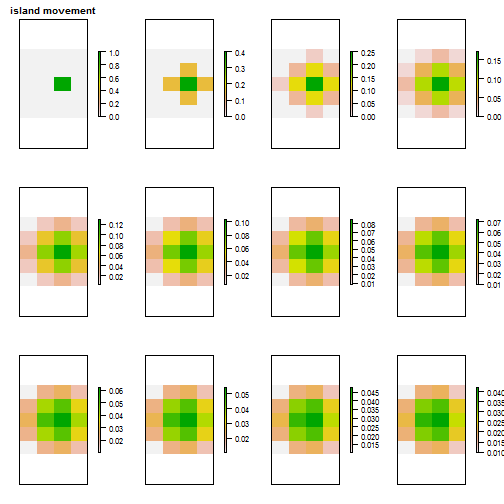
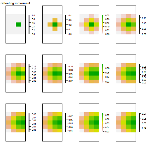
In the first plot, island movement, a pattern of higher density at the centre is retained, because population is lost from the edges. In the ‘reflecting movement’ plot, you can see the population building up at the edges where the expanding population meets them and is reflected back. In time ‘reflecting movement’ leads to an even distribution on the grid.

As an aside. In both examples I used a non-square grid with the starting population slightly off-centre. I do this because experience has shown that using a square grid can hide array referencing bugs in your code. Using a non-square grid for tests and examples helps find these sooner.

I’ve now also modified these movement functions to account for no-go areas and vegetation effects on movement. I’ll describe these in a later post, in the meantime you could look at the rtMove* functions in my rtsetse repository.

As ever, any comments or suggestions of how this could be done differently are welcome.